Obsidian / Graph view
Select the display range and return to the textUse the graph view in Obsidian
Narrow the view and check connections
This page was machine-translated from Japanese. Read the Japanese original
After opening the graph, select the range of notes you want to see first. I checked the search by folder tag, the display of isolated notes, the color group, and the depth of the local graph in a small author-created vault.
Choose the whole and nearby notes according to the range you want to see
Use the global graph to search for the entire library, and select the depth of the local graph to view the surroundings of the open note. The color group is a display that identifies the notes that meet the selected conditions. Open the note to confirm that the text and internal links have been saved.
The note name, text, and tag in the example were created by the author. It is not taken from the actual records of research and life, or from the user's storage. The display position is a layout, not a value that indicates the time required or the degree of understanding.
See Examples of creating, connecting, moving, and re-displaying cards in Canvas for steps to display the relationship by yourself.
Saved contents and display conditions of this example
First, we prepared six Markdown. " The three notes of "research" are entrance → hypothesis → verification, and the two notes of "life" are connected by shopping → eating and internal links, and there is no link to other notes in isolated notes. It is a composition for practice that can distinguish between two connected components and one isolated note.
研究/入口.md → 研究/仮説.md → 研究/検証.md
生活/買い物.md → 生活/食事.md
孤立.md

後からGUIで追加: 追加メモ.md → 研究/入口.md
The first six files were prepared before the app was launched, and only the seventh one was created with the actual editor. " #研究 is written in the three notes and additional notes in the "Research" folder, and #生活 is written in the second notebook of life.
The first conditions for global graphs are Search files blanks, Tags OFF, Attachments OFF, Existing files only OFF, Orphans ON. There were no unresolved links. In the future comparison, only the described search, Orphans, and color groups are switched.
1. Add notes and compare the saved content with the graph
Open Open graph view from the left ribbon. At first, it was six notes and three links. Next, I made an "additional memo" with Ctrl+N and entered the name and text into the actual editor. The saved full text is the following 92 bytes.
# 追加メモ

GUIで追加する著者作成ノートです。 [[研究/入口]]

#研究
When I waited for automatic saving and opened the graph, it became seven notes and four links. One more from the additional memo to the 研究/ entrance increased, and the saved Markdown and the internal link resolution results also matched.
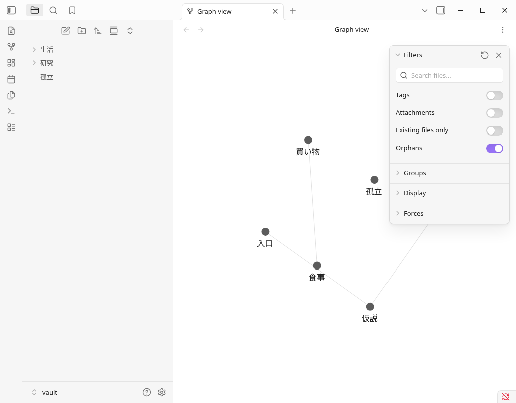
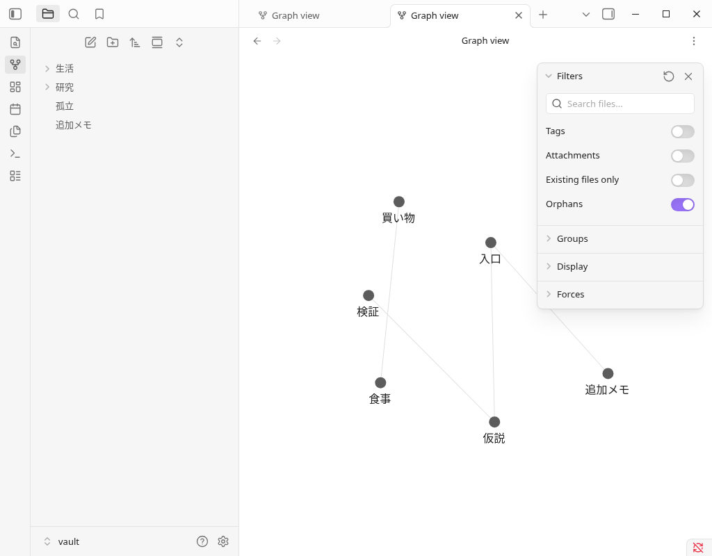
The configuration panel covers some nodes. The number of these two images is a value that has been confirmed by reading the node name and link endpoint from the actual Graph renderer. It is not a counting method that shows all the circles in the image. The image is preserved as it is.
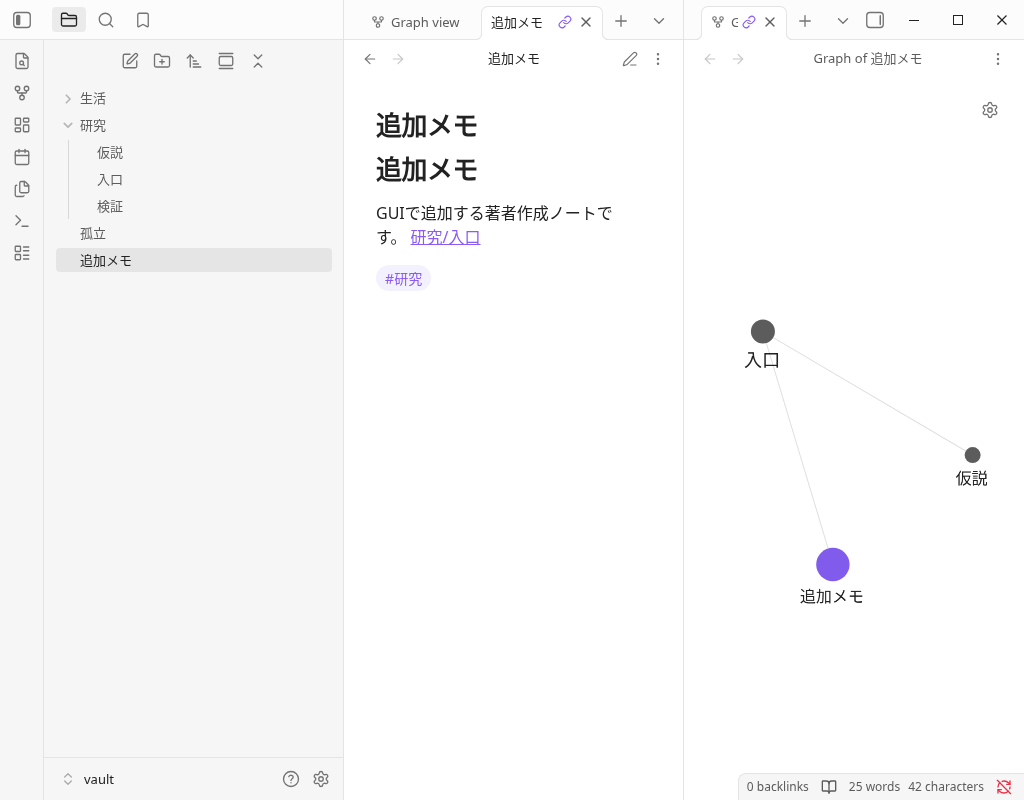
Finally, I reopened the additional notes from the file list and read the text and tags. When adding, after re-displaying, and after the end of the app normally, the saved Markdown had the same content.
2. Choose a different range for folders and tags
Enter a search string in Filters → Search files in Graph settings. path:"研究/" selects notes within a folder; tag:#研究 selects notes containing a tag. The observed results differed as follows.
| Conditions entered | Target notes | Confirmed structure |
|---|---|---|
path:"研究/" | Entry, hypothesis, and verification notes in the 研究 folder | 3 Note / 2 Link |
tag:#研究 | The above three notes and the additional notes directly below the storage room | 4 Note / 3 Link |
| Empty the search string | All seven notes this time | 7 Note / 4 Link |
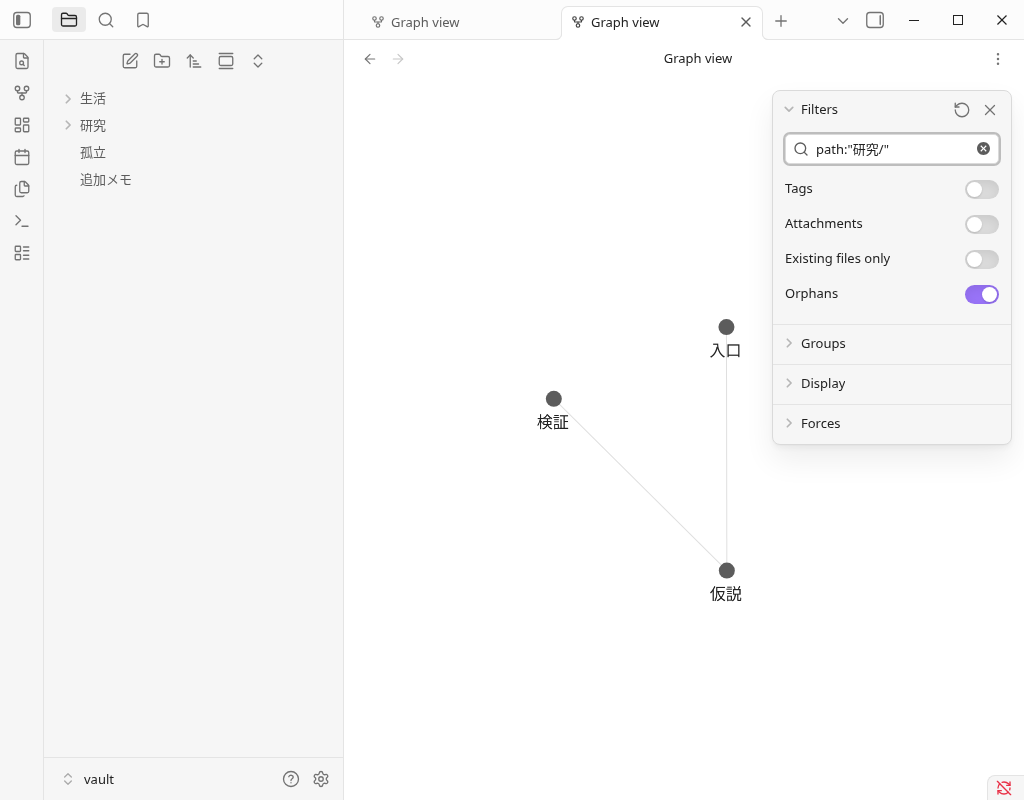
The additional note is at the vault root, so it does not match the path condition for the 研究 folder. It does match the tag condition because it has #研究. We left Tags off in this test and did not test displaying tags themselves as nodes.
When you finish narrowing down, empty the Search files. This time, when the search candidate overlapped with the operation, I closed it with Esc and then clicked the next switch. The folder name and tag name will be adjusted to your saved content.
3. If you also want to see isolated notes, turn on Orphans
With the search string empty, if you turn off Orphans of Filters>, 孤立.md disappears and becomes six notes and four links. When I returned to ON, I returned to the Seven Notes and Four Links, including 孤立.md. Both link endpoints are the same.
In this example, the saved orphan note had no internal links, so toggling the setting changed which notes were shown. If a note is missing, check separately whether its body is saved and which search and display conditions the graph currently uses. Unresolved links and every combination of filters were not tested.
4. Identify notes that match the conditions by color group
Groups → New group, and entered path:"研究/" in the first and tag:#生活 in the second. Click on the color circle of the group and change the first one to RGB 30 / 140 / 220 (#1e8cdc) on the Linux color selection screen. The second assigned color was #d6ad5c.
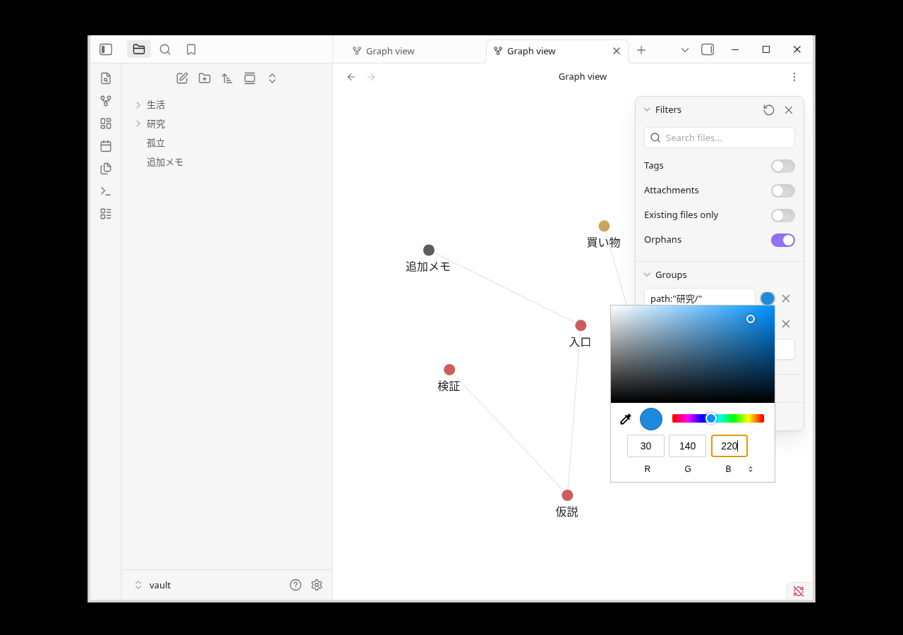
The three notes in the 研究 folder appeared blue, and the two notes with the life tag appeared gold. The additional note at the vault root and 孤立.md matched neither condition, so they received no group color. We also checked the node names and colors; the overall total remained seven notes and four links.
The original image shows the actual color picker. We used the existing X11 mouse and keyboard helpers for GUI input; we did not set the color through the app’s API or by assigning DOM values. Overlapping or reordered color groups, other colors, and other operating systems’ color pickers were not tested.
5 Select a nearby note by the depth of the local graph
Open 研究/入口.md from the file list and select More options → Open linked view → Open local graph in the note. The Filters of the local graph have a Depth slider. The conditions for this time are Incoming links ON, Outgoing links ON, and Neighbor links OFF.
| Depth | Notes included around the entrance | Confirmed structure |
|---|---|---|
| 1 | Entrance, hypothesis referenced from the entrance, additional note referenced from the entrance | 3 Note / 2 Link |
| 2 | The verification referenced from the hypothesis is added to the above | 4 Note / 3 Link |
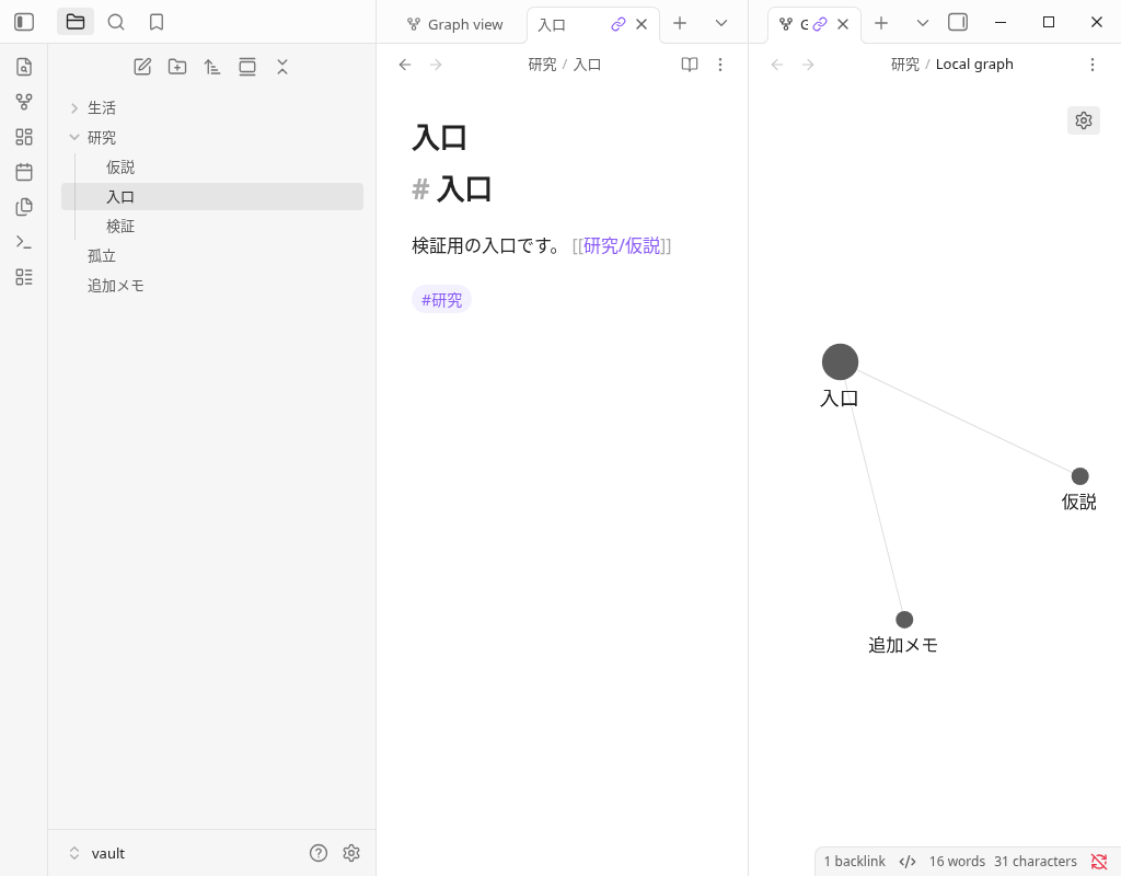
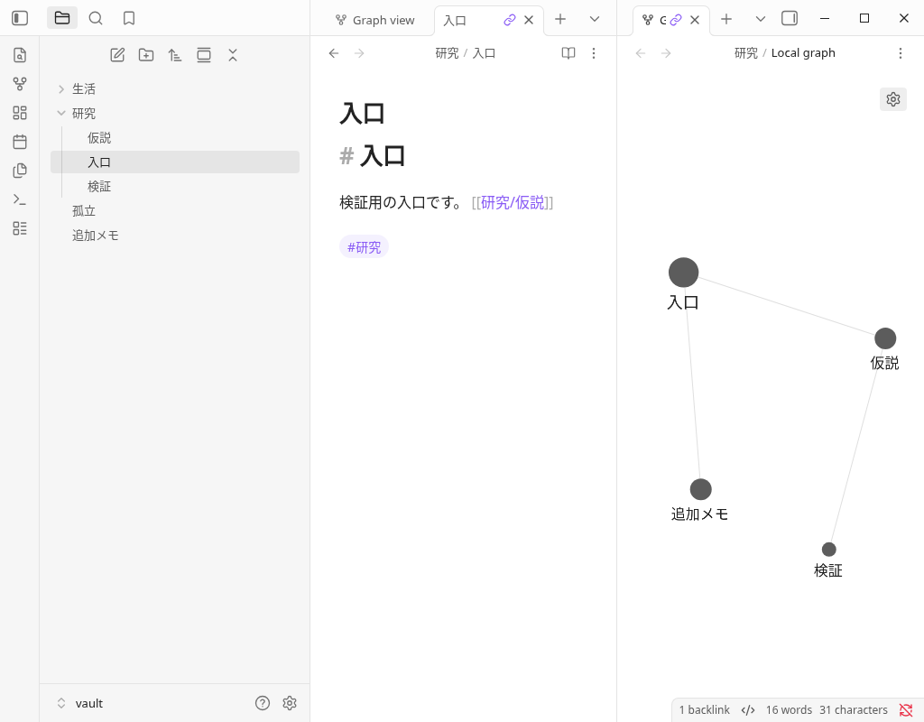
I changed the depth from 1 to 2 with the actual slider operation, and checked the node name and link endpoint. The two notebooks of life and the 孤立.md were not connected to the entrance, so they did not enter these two depths.
Both images are originals captured after choosing the settings and closing the panel. They record depths 1 and 2 for the entry note. Opening a different note also changes the scope of the linked local graph. Depths 3–5 and other combinations of Incoming/Outgoing/Neighbor links were not tested.
Download seven Markdown for practice
The seven files are the same bytes as the original Markdown saved after adding the GUI. ZIP is a distribution package created at the time of preparation for this article, and it retains seven texts and relative paths. In individual downloads, place the folder name and file name of the table together.
Save seven files together (ZIP)
| Relative path in the vault | Original Markdown |
|---|---|
孤立.md | Save 孤立.md |
生活/買い物.md | Save 買い物.md |
生活/食事.md | Save 食事.md |
研究/仮説.md | Save 仮説.md |
研究/入口.md | Save 入口.md |
研究/検証.md | Save 検証.md |
追加メモ.md | Save 追加メモ.md |
SHA256 of the relative path and text of the seven files with the ZIP expanded were compared with the original. ZIP import on the reader's side, placement in other vaults, and delivery from public servers are not included in the verification of the actual application.
Frequently Asked Questions
What do you check when you can't see a note in the graph?
What is the difference between global graphs and local graphs?
Is it the same operation to switch Tags and tag: search?
If there are more nodes and lines, can you judge that you have high knowledge and productivity?
Verification environment and confirmation range
- Actual application:Linux version Obsidian 1.13.7, installer 1.13.7. A small Japanese repository created by the author without community plug-ins.
- Real GUI: Open a graph, create, enter, and save a new note, search input, Orphans switching, group creation and color selection, open local graphs from the file list and menu, Depth slider, re-display, General setting, and normal termination.
- Auxiliary: I prepared the initial six Markdown before starting, and read the saved file, the result of the internal link resolution, the node name, number of lines, color, and settings of the renderer. Adding notes and changing display conditions are real GUIs.
- Image: The original PNG of the real screen is posted without processing. There is a record that the configuration panel and the narrow display area cover some nodes, and the number of cases are compared with the specified API reading value.
- Unverified: iOS/Android/Windows/macOS, Sync, SimpleMemo collaboration, separate terminal, large vault, all search and display settings, speed, learning and productivity, inflow effect.
The actual operation date is October 1, 2026 (Japan time), and the recorded UTC date is September 30, 2026. The original reading record, the correction of the auxiliary code, and the correspondence of saved files and original images will be summarized in verification record.
Official explanation confirmation address
- Obsidian Official Help: Graph view — Description of Filters, Groups, and Local Graph.
- Obsidian Official Help: Search — Description of path: and tag:.
It distinguishes between the description of the fixed official source and the finite actual operation on this Linux. It is not the result of actually trying out all the functions in the official description. This site is a developer site that introduces the independent app "SimpleMemo" and is not an official article of Obsidian.